Microwave control of superconducting cavity and qubit

Group members

LI Yifan e0653565@u.nus.edu

Zhao Luheng e0647245@u.nus.edu

Introduction

Circuit QED is the study of the interaction between light confined in a cavity or resonator and artificial atoms. Usually, the artificial atom is denoted as the qubit, an essential element in the superconducting circuit. We expect to control its ground state and the first excited state for the qubits, which provides a well-defined two-level system. In the past decades, we have witnessed enormous progress in technology and control over the quantum system. With these state-of-art engineering technologies, the superconducting circuit architecture is a powerful platform to explore quantum physics and can serve as a testbed for quantum information,

We have two aluminum 3D superconducting cavity samples A and B, both embedded with transmon qubit chips inside our setup. We have deposited these two samples on the bracket of the MXC stage in the Bluefors dilution refrigerator, which provides a frigid environment with a temperature down to 10mK. In this case, the environmental thermal noise can be suppressed, while the quantum effects of mesoscopic objects, e.g., transmon qubit, non-classical photon state in the cavity, emerge from the measurement. At the same time, quantum technologies enable the manipulation and engineering of these quantum states.

This project intends to characterize the properties of superconducting cavities and the transmon qubits and perform the measurement of qubits. This characterization project will observe the readout resonator spectroscopy, the qubit spectroscopy, and the frequency shift of the readout resonator caused by the qubit state. Further, we can obtain the appropriate power level to implement the readout pulse, the coupling strength between transmon qubit and cavity $\chi$. Then we can perform the Rabi oscillation experiments: Power Rabi and Time Rabi. From these two types of Rabi oscillation, we can find the exact pulse amplitude and pulse length to calibrate the $\pi$-rotation pulse and $\pi /2$-rotation(e.g. $X(\pi )$, $X(\pi /2)$). Once we have the ability to perform a $X(\pi )$ and $X(\pi /2)$, we can execute the $T_1,T_2^{\star }$ measurement protocols to obtains these features of the qubit. We will benefit from this characterization when we accurately engineer the qubit state by the microwave pulse.

Setup

Setup

RF system

A schematic description of the connectivity between the OPX and the experimental system mounted in the low dilution refrigerator. The OPX is a quantum device integrated with FPGA, DAC, and ADC. The analog outputs send the I and Q signals at the range of MHz, which will be modulated by the IQ mixer. to upconvert to the appropriate microwave signal

A schematic description of the connectivity insides the fridge. The BlueFors fridge provides an extremely low temperature (around 10mK) at the MXC flange where the experimental sample is mounted.

Hamiltonian

The quantum system is composed of a transmon qubit and a readout resonator, with the following Hamiltonian

$H=\frac{\hslash }{2}{\omega }_q{\sigma }_z+\hslash {\omega }_r{a}^{†}a+\hslash g(a^{†}{\sigma }^{-}+a{\sigma }^{+}).$

The quantum system works in the dispersive regime where the qubit is strongly detuned from the oscillator with $|\Delta ={\omega }_q-{\omega }_r|\gg g$. There, the Hamiltonian is approximated as

$H_{\mathrm{d}\mathrm{i}\mathrm{s}\mathrm{p}}\approx \hslash {\omega }_r{\hat{a}}^{†}\hat{a}+\frac{\hslash }{2}({\omega }_q+\chi ){\hat{\sigma }}_z+\hslash \chi {\hat{a}}^{†}\hat{a}{\hat{\sigma }}_z,$

The third term, i.e., dispersive coupling term, represents the qubit-state dependent shift of oscillator frequency, or equivalently, a photon-number dependent frequency shift in the qubit spectroscopy, which is also denoted as the ac-Stark shift. Due to the dispersive coupling, the qubit frequency is dressed by a Lamb shift corresponding to the second term in this equation. There, the cross-Kerr nonlinearity strength $\chi$ is derived from the coupling strength $g$ as

$\chi =\frac{g^2}{\Delta }.$

When we send the resonator driving pulse and the qubit driving pulse to the system, the Hamiltonian is given as

$H=H_0+\hslash s(t){\sigma }_x+\frac{m(t)}{2}(a^{†}{e}^{-\omega t}+a{e}^{-\omega t}),$

where the second term rotates the Bloch vector of the qubit around the axis which has an angle $\varphi$ from the x-axis on the x-y plane, namely Rabi oscillation of the qubit. The details are shown in the experiment section.

Experiments

IQ mixer calibration

The IQ mixer suffers from two major drawbacks: one is the IQ imbalance, and the other is DC offset. Hence the calibration and the control of imbalance are essential to limit the signal modulation error. We should pass the proper amplitude and phase correction and DC-offsets to the OPX to calibrate them in our setup. A more detailed discussion of IQ imbalance refers to the reference.

Theoretical analysis

For an ideal mixer with a local oscillator (LO) with the frequency of $\Omega$, the LO signal is described as

$A_{LO}(t)=\mathrm{R}\mathrm{e}[A_0{e}^{-\Omega t}],$

while the RF signal emitted from the IQ mixer is modulated by the I Q signals denoted by $z(t)=z_I(t)+i{z}_Q(t)$. Hence, the RF signal is represented as

$A_{RF}(t)=Re[z(t)A_0{e}^{i\Omega t}]=A_0(z_I(t)\cos (\Omega t)-z_Q(t)\sin (\Omega t))$

The IQ mixer multiplies the I signal by the cosine of the LO, as well as the Q signal by the sine of the LO. In the frequency domain, the RF port generates two sidebands at the two sides of $\Omega$. When we regard the lower sideband is the signal, the upper sideband becomes the image component that needs to be suppressed by a proper choice of $z(t)$. IQ imbalances occur due to the mismatches between the parallel in-phase (I) and quadrature (Q) signal paths. In this case, a non-ideal RF signal is described as

$A_{RF}(t)=Re[z(t)A_0[\cos (\Omega t)+i{r}_{up}\sin (\Omega t+{\varphi }_{up})]],$

where $r_{up}$ and ${\varphi }_{up}$ are the relative amplitude and phase mismatch between the two branches.

Another feature that needs to be calibrated is the LO leakage. For a non-ideal mixer, the LO signal leaks into the RF path, resulting in unwanted components at LO frequency. Therefore, including the effect of LO leakage, the RF signal is given as

$A_{RF}(t)=Re[z(t)A_0[\cos (\Omega t)+i{r}_{up}\sin (\Omega t+{\varphi }_{up})]+ϵA_0{e}^{-\Omega t}].$

The effect of IQ imbalance places an imbalance matrix on the I Q inputs, such as

$\left(\begin{array}{c}{\tilde{z}}_I(t)\\ {\tilde{z}}_Q(t)\end{array}\right)=\left(\begin{array}{cc}(1+{\epsilon }_a)\cos \left({\epsilon }_{\varphi }\right)& -(1+{\epsilon }_a)\sin \left({\epsilon }_{\varphi }\right)\\ -(1-{\epsilon }_a)\sin \left({\epsilon }_{\varphi }\right)& (1-{\epsilon }_a)\cos \left({\epsilon }_{\varphi }\right)\end{array}\right)\left(\begin{array}{c}{z}_I(t)\\ z_Q(t)\end{array}\right).$

Correspondingly, the correction matrix is the inverse of this imbalance matrix. Adding a constant term to $z(t)$ can cancel the LO leakage term. Applying the appropriate gain and phase offsets to the I and Q channels can remove the image term. These offsets and corrections will be passed to the OPX.

Mixer tunning setup and protocol

As seen in the schematic diagram of the RF system, the RF signal is connected to a power splitter whose one branch sends the signal to the fridge input port. At the same time, the other is attached to the spectrum analyzer, detecting the RF output signal. The I Q ports of the IQ mixer receive the I and Q signals from the OPX correspondingly, attenuated by a 10dB attenuator to fulfill the power limitation. We implement the optimization algorithm in the calibration process, which tries different IQ DC-offset and IQ imbalance correction and minimizes them using scipy.optimize.minimize function to lower down LO signal and the image sideband signal.

Error creating thumbnail: Unable to save thumbnail to destination

Figure: mixer tuning setup, which is a part of the RF system. The physical instruments are labeled in red rectangles, and the different ports of the IQ mixer are labels in blue rectangles. Hence we can detect the signal generated from the IQ mixer and find proper DC offsets and IQ imbalance correction.

Result

• 
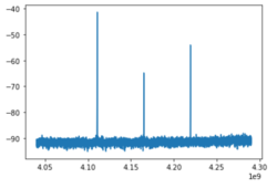  Figure.1 The signal coming from the IQ mixer for controlling qubit before the mixer tunning operation
• 
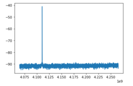  Figure.2 The signal coming from the IQ mixer for controlling qubit after the mixer tunning operation

• 
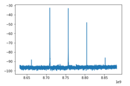  Figure.1 The signal coming from the IQ mixer for controlling readout resonator before the mixer tunning operation
• 
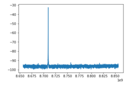  Figure.2 The signal coming from the IQ mixer for controlling readout resonator after the mixer tunning operation

We can observe that after the mixer tuning, the leaked LO signal and unwanted sideband(high sideband in our experiments) are suppressed under the background noise. We obtain the DC-offset value and IQ imbalance correction for I Q ports and pass them to the OPX in each experiment.

One tone spectroscopy

The interaction between the cavity mode and the qubit model can shift the cavity frequency based on the qubit state; moreover, the frequency shift is determined by the coupling strength between the cavity and qubit. For a new sample, we don't know the qubit frequency to manipulate it carefully. Fortunately, even we have no prerequisite knowledge about the qubit. We can observe this frequency shift caused by the coupling of cavity and qubit.

Spectroscopy measured by VNA

By using the Vector Network Analyzer (VNA), we can observe the cavity resonance at the scattering parameters $S_{21}$. We can compare cavity frequency with different sweep signal power and see if the frequency shifts. In the high-power mode, we send a vast number of photons into the cavity, which essentially overwhelms the effect of the qubit, resulting in the measurement of the bare frequency of the readout resonator. In contrast, the qubit is in its ground state $|g⟩$ in the low-power regime, the cavity frequency is dispersively shifted due to the ground state of the qubit $|g⟩$. Since the $\Delta$ between the cavity frequency and the qubit frequency is large, we can ensure that when the cavity is driving (the VNA signal sweeps around the cavity frequency), the qubit can be maintained at the ground state in the low-power regime.

A bigger frequency shift means a stronger coupling between the cavity and the qubit exists. The frequency shift of the cavity is a rough estimation of the coupling $\chi =g^2/\Delta$ rather than the exact value.

Resonator spectroscopy

We can also use the OPX device to realize the spectroscopy function. When we execute the readout pulse and sweep its frequency, the response of the readout resonator on the frequency-sweep readout pulses will cause different amplitudes. Therefore, the amplitudes of the signal coming from the readout resonator at different frequencies form the resonator spectroscopy.

OPX program

The program resonator_spectroscopy consists of an outer averaging loop and an inner scanning loop. The inner loop scans a range of frequencies and in each cycle changes the frequency using the update_frequency command, and then measures the readout resonator using measure command. wait is implemented to let the resonator relax to its vacuum state.

Resonator spectroscopy with qubit being ground state

Resonator spectroscopy with qubit being excited state

Low-power resonator spectroscopy comparison

Readout power and frequency 2D sweep

Two tone spectroscopy

Principle

We do not send a signal with the qubit frequency to the quantum system to obtain qubit spectroscopy and acquire its response. The protocol to realize qubit spectroscopy is to extract the qubit information via the coupling between the readout resonator and the qubit. From the resonator spectroscopy section, we have known that the different state of the qubit shifts the resonator frequency or causes different signal amplitude in the same frequency. Therefore, obvious amplitude contrast can realize a measurement of the qubit state, further the qubit spectroscopy when we scan the frequency of qubit saturation pulse.

There are two kinds of measurement protocol that we can harness: one is the low-power readout that we use in the following experiments, the other is the high-power readout. We chose a Gaussian pulse in the low-power readout setting whose relative amplitude of 0.04 (compared with the initial 0.32V amplitude). Besides, the length of the readout pulse is 1.2us, and the frequency of the readout pulse is the readout resonator frequency shifted by the ground state of the qubit in the corresponding power. In the 2-dimension power and frequency sweep shown in the last section, the amplitude represents the qubit's state at this low-power readout resonator frequency.

OPX program

The control program qubit_spectroscopy consists of two loops: the outer loop used for averaging and the inner used for the frequency sweep. In each cycle of frequency sweep, we update the qubit's frequency and implement a corresponding saturation pulse which ensures that qubit being the excited state. Then we align the qubit and readout resonator and wait for the saturation pulse to be done. Afterward, we execute a long readout pulse to the readout resonator and save the IQ components. We use the low-power readout pulse whose frequency equals resonator frequency with qubit being $|0⟩$ at corresponding readout pulse power. The contrast of received readout amplitudes between the ground state $|0⟩$ and the excited state $|1⟩$ represents the qubit spectroscopy.

Coarse frequency scan

We implement a coarse frequency scan to find the approximate qubit frequency.

• 
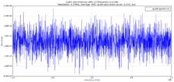  Figure.1 LO frequency 4GHz
• 
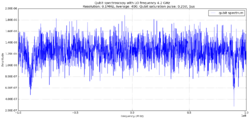  Figure.2 LO frequency 4.2GHz
• 
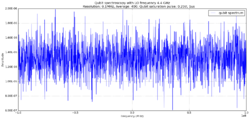  Figure.3 LO frequency 4.4GHz

• 
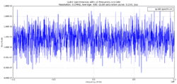  Figure.4 LO frequency 4.6GHz
• 
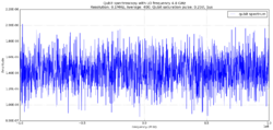  Figure.5 LO frequency 4.8GHz
• 
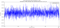  Figure.6 LO frequency 5.0GHz

From the coarse frequency scan, we find that the qubit frequency is around 4.1GHz. Then we can narrow the frequency range and increase the frequency resolution to search the exact qubit drop. We also observe a small drop that is symmetric around the LO frequency compared to the qubit drop. The reason for this signal needs to be studied later.

Precise qubit spectroscopy

We do precise qubit spectroscopy from IF frequency -60MHz to -40MHz with the LO frequency 4.165GHz.

In this spectroscopy, the lowest point corresponds to the excited state of the qubit, which shows an amplitude of around 0.7E-6, while the flat signal around 1.3E-6 represents that the qubit is in the ground state. Besides, we obtain a more precise qubit frequency, that is, 4.111GHz.

In the following, if we want to drive or implement the qubit, we should introduce the qubit drive pulse whose frequency is the same as the qubit frequency.

Rabi sweeps

One- and two-dimensional Rabi sweeps are critical qubit characterization protocols. In this section, we perform the power Rabi pulse sequence and time Rabi pulse sequence to find the right amplitude and time of pulse to execute a particular single-qubit gate, such as $\pi$-pulse around the x-axis which rotates the ground state $|g⟩$ to the excited state $|e⟩$ and vice versa.

The control pulse follows

$s(t)=A(t)\cos ({\omega }_{d}t+\varphi ),$

where $A(t)$ is the time-dependent amplitude of the pulse. When the drive frequency is detuned from the qubit as $\Delta ={\omega }_d-{\omega }_q\ne 0$, it allows the rotations around the z-axis in the Bloch sphere. When the drive frequency is the same as the qubit frequency, the qubit rotations around an axis in the x-y plane, which is defined accordingly to the phase $\varphi$. For the rotation around the x-axis, the phase is set as 0, and the rotation angle is given

$\theta ={\int }_{t_0}^{t_0+\tau }A(t)dt,$

where $t_0$ is the time at which the pulse starts and $\tau$ is the duration of the pulse.

Power-Rabi experiment

In the Power-Rabi experiment, we fix the drive pulse duration and sweep the power of the drive pulse. The sequence

• Prepare the qubit to the ground state $|g⟩$, which is realized by a long wait time allowing the qubit is relaxed to its ground state.
• Execute a gaussian shaped pulse with a fixed duration $\tau$ and varying peak amplitude $a$ which rotates the qubits by $\theta \propto a\times \tau e^{-{\tau }^2/2{\sigma }^2}.$
• Execute a weak readout pulse to the readout resonator, which is coupled to the qubit. From the phase of the reflected pulse, we can deduce the state of the qubit.

With the qubit drive pulse, the state of the qubit evolves as $\cos (\theta )|0⟩+\sin (\theta )e^{i\varphi }|1⟩$, hence the probability of measuring the state $|1⟩$ is $P_{|1⟩}=|{\sin }^2\theta |$. To obtain an obvious result, the above sequence is repeated large times, therefore, the measurement sample is averaged.

We can use this Rabi experiment to calibrate any signal qubit rotation gate that rotates the qubit by an angle $\theta$ around a rotation axis which is rotated from the x-axis on the x-y plane, namely $R_{\varphi }(\theta )$, e.g., $\pi$-rotation and $\pi /2$-rotation. However, the $\varphi$ cannot be determined from the Rabi oscillations.

• 
• 

Time-Rabi experiment

In the Time-Rabi experiment, we fix the drive pulse amplitude and sweep the drive pulse length.

In this figure, with the varying pulse length, there is a platform of amplitude at the beginning from 0 to 150ns, representing that the qubit is still in the ground state. One of the possible speculations is that the drive pulse is so week that it cannot excite the qubit, leaving it in the ground state. After 150ns, the I and Q data show a clear sinusoidal waveform. We can find the proper fit for these data as well. From the analysis, the gaussian pulse of 900ns length with amplitude 0.32V, $\sigma$ is 1/6 of pulse length can realize the $\pi$-pulse of the qubit.

T1 measurement

Measurement protocol

We play a $\pi$ pulse to rotate the qubit from the ground state into the excited state. The qubit will be relaxed from the excited state with respect to the time. Hence, at different time points after the $\pi$-rotation of the qubit operation, we execute the readout pulses and obtain the probabilities $P_{|1⟩}$ of the qubit being excited state. The probabilities $P_{|1⟩}$ decay from 1 to 0 in terms of time.

This figure shows the pulse sequences for $T_1$ measurement for the transition between the gound state and the excited state. $\pi$ represents the $\pi$-pulse and $\Delta t$ denotes a variable time delay. After the $\pi$-pulse on the qubit, the probability of finding the qubit to be the excited state has an exponential decay proportional to $e^{-\Delta t/T_1}$.

Experiment

Based on the previous Rabi oscillation experiments, we use a gaussian pulse whose pulse length is 900ns, $\sigma$ is 150ns and the initial signal voltage is 0.25V, corrected by an amplitude ratio of 0.938 to implement the $\pi$-rotation. This operation flips the qubit from the ground state to the excited state. According to the readout resonator spectroscopy with varying power, we use a low-power readout pulse to perform the measurement. The initial settings of the readout pulse are 0.32V, rectangle waveform, 1200ns pulse length. Correspondingly, the low-power readout implements an amplitude correlation with the ratio of 0.04. The probabilities of qubit to be in the excited state will display on the different amplitude contrasts of returned readout pulses.

In the $T_1$ measurement, we sweep the duration between $\pi$-pulse and the readout pulse. Besides, we repeated the same pulse sequence 5000 times for each relaxation time and averaged the measured results. The averaged data are shown as the blue dots in the below figure. The red curve depicts an exponential fit for the data, which gives an expectation of $T_1=80\mu s$.

Ramsey measurement

The Ramsey sequence follows

• Apply a $\pi /2$-pulse to the qubit, which prepares the qubit in the superposition state.
• Wait for time $\Delta t$ that is swept to
• Apply another $\pi /2$-pulse to the qubit.
• Perform the readout pulse.

For the qubit $\pi /2$-pulse, the frequency is artificially detuned from the exact qubit frequency by $\delta$. In the ideal case, the probability for the qubit to be in the excited state after the two $\pi /2$-pulse intersected with a wait time $\Delta t$ oscillates as a function of the artificial detuning $\delta$ and the time delay $\Delta t$ as

$P(|1⟩)=\frac{1}{2}(1+\cos (\Delta t\delta ))$

In practice, we use the qubit frequency from the spectroscopy denoted as ${\omega }_{spec}={\omega }_{ge}-{\delta }^{\prime }$. Combing with the detuning $\delta =|{\omega }_{pulse}-{\omega }_{spec}|$, the qubit transition frequency can be extracted as

${\omega }_{ge}-{\omega }_{spec}-{\omega }_{Ramsey}+\delta$

However, the repetition and averaging of Ramsey measurement will result in ${\omega }_{spec}={\omega }_{ge}$, and a trace oscillating at $\delta$ will be observed. Due to the dephasing of the qubit, we can observe that Ramsey oscillations have an exponentially decaying envelope proportional to $e^{-\Delta t/T_2^{\star }}$, where $T_2^{\star }$ is denoted at the averaged dephasing. The relation between averaged dephasing time and the pure dephasing time is given as

$\frac{1}{T_2^{\star }}=\frac{1}{2T_1}+\frac{1}{T_{\varphi }}$

where $T_{\varphi }$ is the pure dephasing and $T_1$ is the energy relaxation time. Ramsey measurement applies an average over a large number of equivalent measurements, resulting in the averaging of the fluctuations of the transition frequency. The real dephasing time $T_2$ that measured by the Ramsey echo is usually larger than $T_2^{\star }$